This chapter is part of the TwinCAT 3 Tutorial.

In this section I’m going to introduce you to one of the most powerful tools in your debugging arsenal: the TwinCAT 3 Scope View. This is a software-based digital oscilloscope that comes free with TwinCAT 3.

Create a Test PLC Project

First, create a PLC project for testing. I’m going to describe a simple scenario that generates a sine wave at a reasonably high frequency. Follow these instructions (assuming you’ve read the rest of the tutorials and you’re familiar with how to do this):

1. Create a new TwinCAT 3 solution
2. Use the wizard to create a standard PLC project (called PLC1)
3. Setup the SYSTEM->Real-Time node (hint: “Read from Target“)
4. Setup SYSTEM->Tasks->PlcTask to run at 1 ms
5. Remove the structured text MAIN program and create a new ladder logic MAIN program
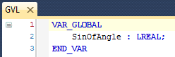
6. Create a global variable list called GVL

Here’s the contents of the GVL:

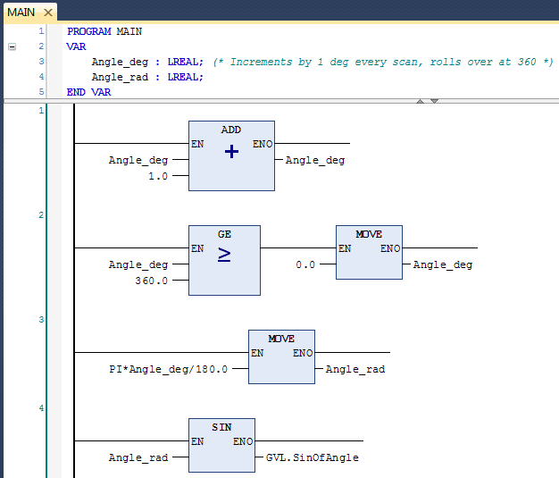
Here’s the MAIN program:

Now build and activate the configuration. Go online and make sure you can see it running.

Add a TwinCAT Measurement Project

The TwinCAT 3 Scope View is built into the Visual Studio 2010 shell. You use it by first creating a new “TwinCAT Measurement Project.” In the Solution Explorer, go to the top level (Solution) node and right click on it. Select Add->New Project… from the context menu. That will open the Add New Project dialog:

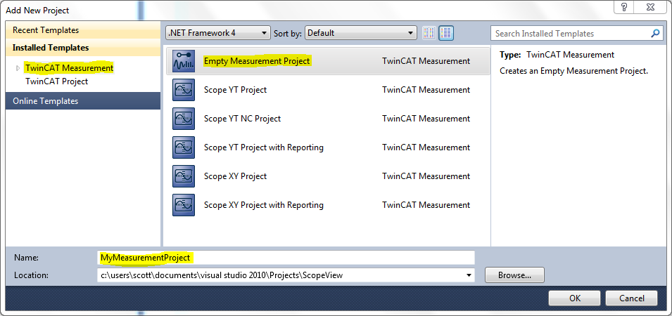
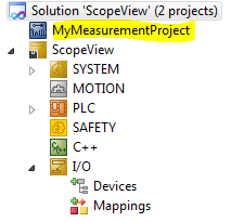
Make sure you have TwinCAT Measurement selected in the upper left under Installed Templates. Then select Empty Measurement Project in the middle panel, and give it a descriptive name in the Name field. Click the OK button to create the project. Now you’ll see the new project under your solution node in the Solution Explorer:

Add a Scope to your Measurement Project

Now you have to add a Scope. There are two basic scope types: YT and XY. A YT scope plots some variable on the vertical Y axis and time along the horizontal (X) axis. An XY scope plots two variables against each other, one on the X and one on the Y axis. In our case we want a YT scope.

In the Solution Explorer, right click on your new measurement project and select Add->New Item… from the context menu. That will open the Add New Item dialog window:

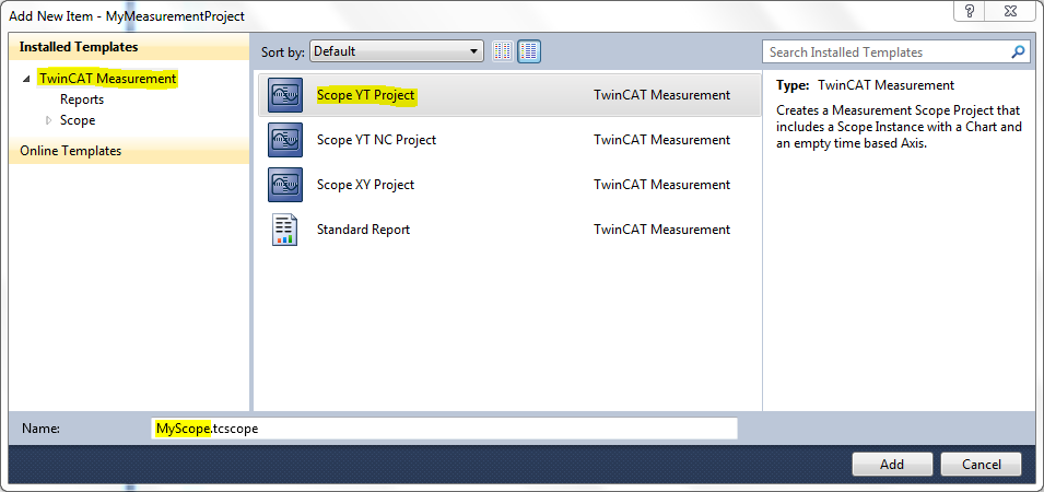
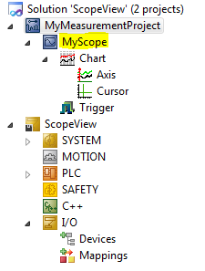
With TwinCAT Measurement selected in the upper left under Installed Templates, select Scope YT Project in the middle panel, add a descriptive name for your scope in the Name box, and click Add. Now you’ll see a new scope node under your measurement project in the Solution Explorer:

Adding Variables to your Axis

Start by adding the GVL.SinOfAngle variable to the Axis that was created by the wizard. Right click on the Chart->Axis node under your scope in the Solution Explorer and choose Target Browser from the context menu. That will display the Target Browser window:

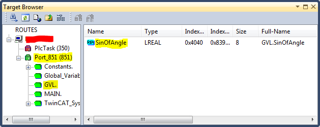
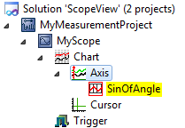
At first it will show the ROUTES node, and under it you should see your PC name (where the red box is in the figure above). Click on your PC name, expand Port_851, click on the GVL. node, and you will see SinOfAngle in the right pane. Double-click on SinOfAngle and it will add that variable to your Axis. Then close the Target Browser window. Now you’ll see SinOfAngle added to your Axis under the Solution Explorer:

Record Data

Make sure you have the scope window visible by double-clicking on the scope node in the Solution Explorer. Now look for the TwinCAT Measurement buttons in your toolbar:

The button on the left is the Record button. The button in the middle is the Stop button. Click the Record button, wait a few seconds, and click the Stop button (and you’ll have to click an OK button on a dialog after clicking the Stop button). Now you’ll have some data to look at:

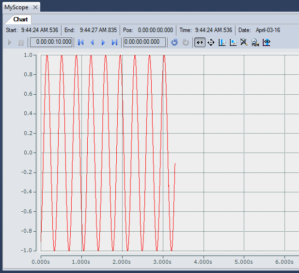
If you want to zoom in on the data, hover your mouse over the point where you’d like to zoom, and use the mouse wheel to zoom in (forward on the mouse wheel zooms in, backwards zooms out). If you don’t have a mouse wheel, look for the Zoom X button on the chart toolbar. Moving left/right is as simple as clicking, holding, and dragging the mouse left or right.

Measuring using Cursors

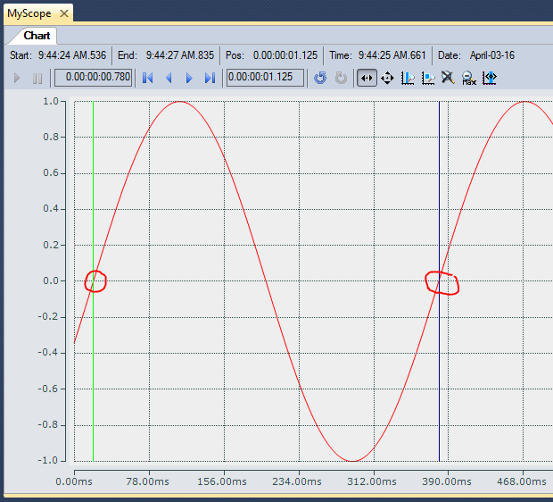
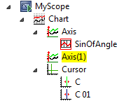
You can take measurements from the scope using X and Y cursors. Let’s say I want to measure the sine wave period, which is the time between one positive (rising) zero crossing to he next positive zero crossing. First we need to create two X cursors. In the Solution Explorer, under the Chart node, find the Cursor node. Right click on the Cursor node and select New X Cursor. Do this twice. You’ll see the two cursors listed under the Cursor node:

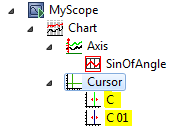
Notice that the C cursor is green and the C 01 cursor is blue (you can barely see it in the icon). You’ll also see new green and blue X cursor lines in the chart itself:

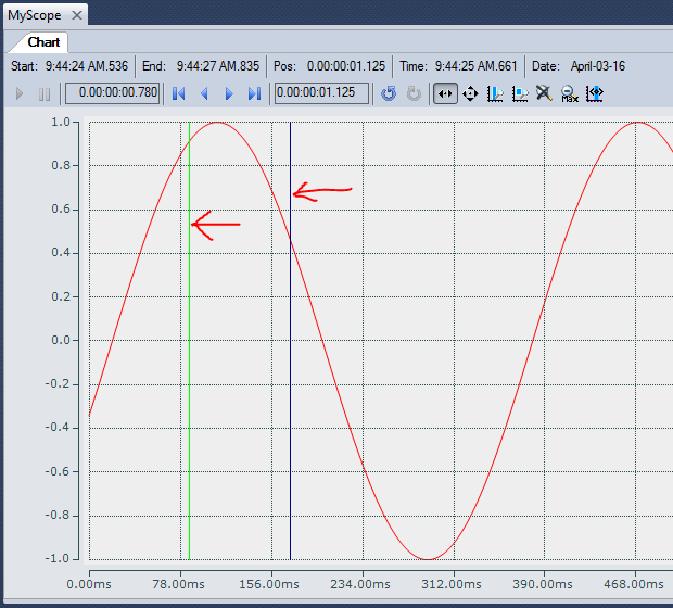
Now click and drag the green cursor to the first positive zero crossing of the sine wave, and click and drag the blue cursor to the second positive zero crossing:

Now right-click on the C node (the actual cursor under the Cursor node) in the Solution Explorer again and select Cursor Window from the context menu. That will display the Cursor window:

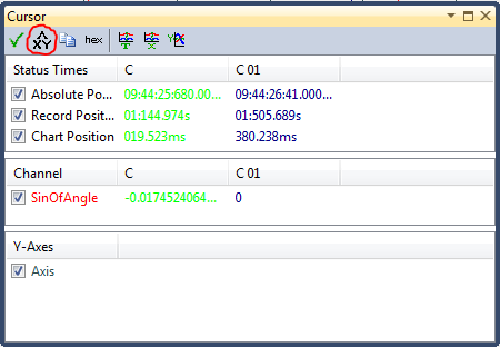
You can see the relevant details of each cursor in the C and C 01 columns. Now click the Delta button (circled in red). That displays another column showing the difference between the two cursors:

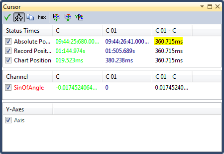
Here we can see the time difference between the two cursors is about 360 ms, which makes sense since the input angle is changing by 1 degree every scan, and each scan is 1 ms long.

Adding More Axes

The sine wave has a Y range of -1.0 to +1.0 in amplitude. Suppose we wanted to compare this to the input angle (in degrees) which ranges from 0.0 to about 360.0 degrees. Plotting them on the same graph would be difficult because the amplitudes are so dissimilar.

To scope variables with different amplitudes, simply add more axes. Right click on the Chart node in the Solution Explorer and click New Axis from the context menu. That will add a new axis called Axis(1). You can rename these axes if you like:

Looking at your chart window, you’ll now see two Y-axes on the left side.

Now right click on the new Axis(1) node and select Target Browser from the context menu. This time use the Target Browser window to add the Port_851->MAIN.->Angle_deg variable to your new axis:

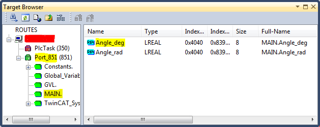
When you do this, it has to delete the captured data and it asks if you want to save the data to a file first. Just say “no”. Close the Target Browser window.

Now use the Record and Stop buttons to record a few seconds of data again:

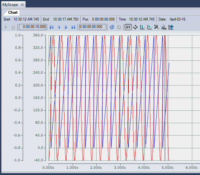
The chart looks a little more cluttered with two axes overlaid like this. Zooming in helps a little. However, I generally prefer using “stacked Y axes.” You can enable this feature in the chart properties. Right click on the Chart node in the Solution Explorer and choose Properties from the context menu. Now scroll down to the bottom of the Properties window and look for the Stacked Y-Axes property. Set this property to True. Now your axes will appear “stacked”:

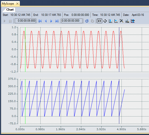
I also find stacked axes useful when scoping boolean variables because I find it easier to see which ones are off and which ones are on at any given point in time.

Conclusion

The Scope View is a powerful tool for troubleshooting irksome transient conditions or measuring high speed signals. Once you know the basics, the interface is fairly user-friendly and best-of-all the tool is included for free with TwinCAT 3.

This chapter is part of the TwinCAT 3 Tutorial. Continue to the next chapter: Part Tracking.