This chapter is part of the TwinCAT 3 Tutorial.
Motion Control is a big topic. Motion Control refers to the use of servo (and stepper) motors in your system. A servo requires a motor and a position feedback device such as a resolver or an encoder, and it controls the position of the motor using a feedback control system.
Motion Control systems are not new, but they have a parallel lineage to PLCs. Since around 2000 we’ve seen more and more convergence of Motion Control and PLC systems, but they are still separately packaged modules within the system. In TwinCAT 3 they are separately licensed modules. The PLC system is licensed as TwinCAT PLC, and the motion control system is called TwinCAT NC. The latter is licensed depending on how many “axes” (i.e. servo motors) your system needs. The base package is 10 axes, and you can add more axes for more money.
The “NC” in TwinCAT NC means “numerical control”. It’s the same NC as “CNC machines”, which can mill (or cut) away material from a block of steel with accuracies better than a thousandth of an inch. In fact Beckhoff originally got its start in motion control systems, so TwinCAT 3 includes one of the better motion controller systems available today.
The TwinCAT NC module is just a basic motion controller that gives you “point to point” motion. That is, each axis is controlled independently. If you need your axes to work in a co-ordinated way, such as in a 3-axis CNC mill where you need to follow a complex path in 3 dimensions, then you need “interpolated motion”. TwinCAT 3 offers this as an add-on to TwinCAT NC, called “TwinCAT NC I”. This add-on actually includes a built-in G-code interpreter. G-code is the language that CNC mills (and FDM-type 3D printers) use to instruct the motion controller on the path to follow to create a finished part.
Industrial robots, such as those from ABB, Fanuc, Motoman, etc., are actually controlled by interpolated motion controllers internally. It’s no co-incidence that Fanuc is both a leading supplier of industrial robots and CNC mill controllers. The technology is similar. In fact TwinCAT 3 does support kinematics packages for industrial robots, and you can even purchase a Codian Delta Robot through Beckhoff and use TwinCAT NC I with a delta robot kinematics package to control the robot directly from TwinCAT 3.
Since motion controllers have evolved from their origins in CNC milling and industrial robots, the sequential nature of their programming (in the form of G-code or proprietary robot programming languages) has never fit well with ladder logic programming, and gives rise to what I call the Ladder Logic/Motion Controller Impedance Mismatch.
In PLC programming it’s typical to think in terms of discrete outputs. Turning on an output can do many things, such as turning on a pneumatic valve to apply air pressure to a cylinder, turning on a motor to run a saw or a pump, or turning on a heater to control the temperature of a fluid. In all of these cases you can think of a discrete output meaning “try to do X.” For instance, “try to extend this cylinder,” or “try to start motor,” or “try to increase temperature.” We normally have feedback mechanism like a proximity switch, or a level or temperature sensor to tell us that our action succeeded. This try/confirm idea naturally gives rise to ladder logic programming patterns like the Five Rung Logic Block and the Step Pattern. Implicit in the Five Rung logic is the idea of “when is it safe to perform (and continue performing) this action?”
Motion controllers, on the other hand, are designed to follow a strict set of sequential instructions, with little consideration of how to recover when things go wrong. Consider the idea of a weld robot. It waits for a part to be loaded, follows a path (series of points) to move the weld tool into position, clamps the welding tool, fires the welder, unclamps, and follows another path back to the home position. The linear nature of the sequence makes this particularly easy to program, but what if someone opens the gate and removes the part while the robot is moving in towards the part? The robot can’t continue the program because the part is no longer there. However, the check for part presence would have been done at the beginning of the program. That means you need to insert a second part presence check right before you clamp the welder, and if it’s not present then skip over the weld and jump to the move-out sequence. Unfortunately this means the robot recovers by continuing in towards the missing part. The “right” thing would be to move back out immediately, but programming a way for the robot to find its way back away from the part without crashing into an obstacle can be quite difficult and complicated. That’s why many industrial robots are tended to by operators who frequently have to enter the cell with a teach pendant and recover by manually “jogging” the robot safely around obstacles back to a known home position.
If the motion was done by a PLC controlling a sequence of air cylinders, the recovery logic would be comparatively simple: just retract them in the right sequence. Typically your “safety” rung in your Five Rung logic block already contains the logic about when it’s “safe” to retract those cylinders without crashing, so if you give them all the trigger signal to retract, they’ll automatically retract in the right order.
When a new control system programmer comes out of school, they always want to program the industrial robots because they look so cool. However, I always tell them, “the robots are stupid but PLCs make them smart.” For a PLC to make a robot smart, it needs to know the current robot (or motion controller) position. If you don’t know where the robot is, how can you program a smart recovery path? Unfortunately, getting the current robot position out of the robot and into the PLC can be difficult at best, and nearly impossible with some older robot controllers. Thankfully, with TwinCAT 3, the motion controller and the PLC are operating in the same runtime, so the PLC automatically has access to all motion controller information, which makes your job a lot easier.
Creating a Motion (NC) Task
To add a motion controller to your TwinCAT 3 project, go into the Solution Explorer and find the MOTION node directly below the SYSTEM node. Right click on the MOTION node and choose Add New Item… from the context menu. That will pop up the Insert Motion Configuration dialog box. Choose NC/PTP NCI Configuration and click Ok.
You can only insert one motion controller. The motion controller automatically defines a task and that task can be scheduled under the SYSTEM->Real-Time node just like your PLC tasks. Typically this should be a high priority task (higher than your PLC tasks) and should run often, such as once every one or two milliseconds, even if your PLC only runs once every 10 milliseconds. This task handles all communication with the servo drives (even for drives from manufacturers other than Beckhoff) and provides a generalized “axis” interface for your PLC to deal with. It can also close the position feedback loop for some less expensive drives that don’t offer a position loop, synchronize multiple axes in an interpolated system, and perform kinematic transformations in the case of industrial robots. It even has a G-code interpreter.
Adding A Servo Drive and Axis
Beckhoff offers a really good line of EtherCAT servo drives in their AX5000 range. It’s also advantageous to purchase a Beckhoff servo motor so you know they’re compatible (and it makes the configuration simpler). In order to size your servo motor you need to start with the performance requirements of your mechanical system (such as load inertia, required rates acceleration, deceleration, speed, and expected duty cycle. I suggest taking this information to your local Beckhoff sales representative and they can help you to size the motors and drives accordingly. When sizing the motor, optimal performance is typically achieved when the load inertia and motor inertia are approximately equal, though in practice this is sometimes impossible. Other mechanical considerations will also factor in: for instance, a belt drive can sometimes give you higher top speeds, but at the expense of lower acceleration and deceleration (due to the belt flexing), so adding more torque won’t help if your mechanical system can’t handle it.
Beckhoff also offers an interesting line of lower cost servo drives that can connect right into the terminal strip of an EK1100 head module. These are limited to around 48V and 4A max, and the position loop is closed in the motion control task rather than in the drive itself, but for lower performance smaller applications these can offer significant cost savings. There is also a line of similar terminal slices for stepper motor control, which offers an even lower cost alternative, if your application doesn’t need servo-class performance.
In Solution Explorer, under the I/O node, go to the point in your I/O tree where you’re going to attach the drive (or you can just do a bus scan too). When you add the drive (manually or with a scan), it will say, “EtherCAT drive(s) added. Append linked axis to NC-Configuration“? If you choose Yes, it will add an axis object under the NC-Task in the MOTION node, and it will link the drive I/O under that axis to the new drive under the I/O node. Typically you would answer Yes when programming a system for the first time.
Here’s what it looks like after I’ve added an AX5118 drive (single axis 18 amp):
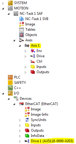
I highlighted the new drive and the new axis. Note that you can (and should) rename the drive and axis to match the real name of your axis in your electrical drawings.
Note that if you expand the Axis->Drive node you’ll see that it’s automatically linked some I/O to the physical I/O under the actual drive:
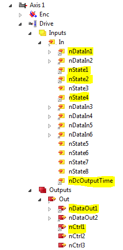
You never have to touch these mappings yourself, even if you’re connecting the drive to the axis manually. Double-click on Axis 1 under the Axes node, and go to the Settings tab. You’ll see where the drive I/O is linked to the axis:
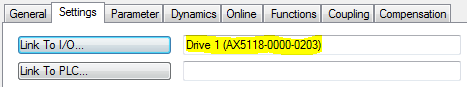
If you click the Link To I/O… button, it’ll give you a list of drives available for linking.
Configuring the Drive
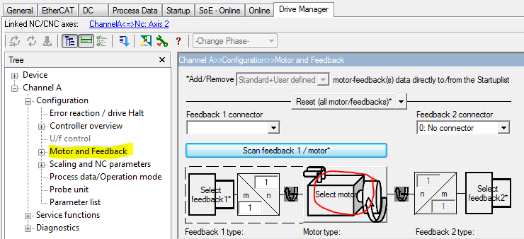
Double-click on the drive under the I/O. All of the configuration is done under the Drive Manager tab. The first thing you want to do is setup the motor and feedback. If you’ve purchased a Beckhoff motor, this is simple. In the tree, go to Channel A->Configuration->Motor and Feedback. Click the Select motor button on the right:
That will open the Select a Motor dialog box. You will need the motor part # from the motor nameplate, or from the motor ordering information. TwinCAT 3 includes a datasheet for each motor, so it knows all the motor characteristics and feedback characteristics. Select your motor and click OK.
TwinCAT 3 will then display a dialog box titled, Power supply and extra settings for:
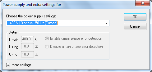
This is a “gotcha”. Most people would think this means you should specify what voltage we’re supplying to the drive, which in the United States would be 480V, 3 phase, 60 Hz. However, since I specified a Beckhoff motor and it was designed for Europe, I actually must keep the voltage set to 400V or I get an error (the voltage has to match the motor voltage). This was several TwinCAT 3 versions ago, so I don’t know if anything has changed since then, so it might be a good idea to check with your Beckhoff representative about this. Of course, these are still power supply settings (relating to the incoming power) so if you set the voltage to 400V with 10% tolerance, and connect it to 480V, the drive will fault because the input voltage is too high. Since the drive (and apparently the motor) is actually 480V tolerant, the “correct” way to handle this situation is to select Other settings, and then manually edit the U+rng setting to 30.0% (this is the maximum value allowed). This will allow your voltage to go up to 520V which is an 8% over-voltage allowance based on 480V. This means the drive will actually work from 360V up to 520V. Here are the settings:
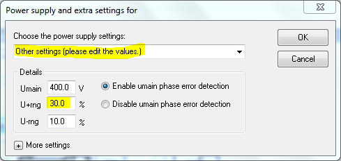
Note: in my latest project (spring of 2016) I was able to specify 480V for all the servo motors, so it looks like Beckhoff has updated the software to fix this problem since I wrote it.
Click OK.
Note that if you’re in Canada, the typical industrial voltage is 600V. Unfortunately this means you’ll have to use a step-down transformer to use these drives. Since there are also many other devices that can run off 480V, it’s typical to step-down to just 480V instead of 400V, and use the settings shown above.
After setting the power supply settings, it will ask if you want to set the scaling and parameters now. If this is your first time adding a motor to this drive, say OK, but if you’ve already modified these parameters and you’re just selecting the motor again (or selecting a new motor), you’ll probably want to say Cancel.
If you click OK, then it will display the Scaling and NC parameters node in the drive manager tree:
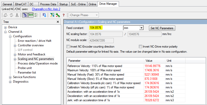
Make sure you set the Feed constant (highlighted). Assuming you’re driving a linear axis of some kind (rail or ball screw), this is the distance that the linear axis moves in one revolution of the motor. As soon as you set it, click the Set NC Parameters button. This will set the defaultNC parameters (below).
You need to set reasonable motion limits for the axis (this is done in the Axis node under Axes, on the Parameters tab). Make sure you do this before trying to move your axis. This will depend on your application. For instance, it sets Maximum Velocity to 100% of the maximum motor speed. However, the mechanical limitations of your machine may not be able to tolerate that speed. You have to calculate that maximum linear speed your system can handle, and set this parameter accordingly. Similarly, set reasonable limits for Manual Velocity (a.k.a. “jogging”). The automatically calculated values are typically much higher than you would want during system testing and start-up. Calibration Velocity is used during the homing routines.
Finally, setup the digital I/O on the drive. Not all drives have Digital I/O, but most at least offer inputs for limit switches. These are important, so let’s take a short detour on the topic of axis limits. An axis can have up to 3 sets of limits:
- Software Limits
- Hardware Limit Switches
- Hard Stops
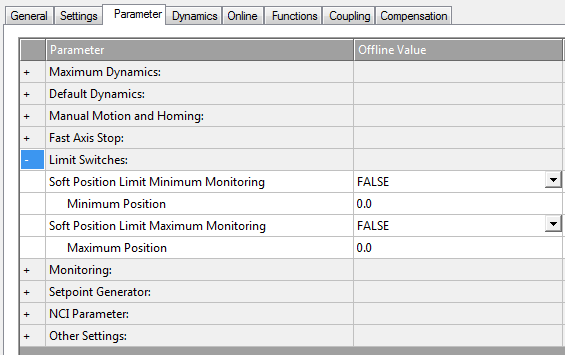
Software Limits are software-only limits on the axis travel. They are practically free, but they’re also the least useful. First of all, software limits are only useful after the axis has been calibrated (homed), so they won’t protect you during system startup, or during the homing operation. Secondly, software limits depend on the motor’s encoder value, so it won’t catch certain classes of failures such as a shaft coupler break, a belt break or a tooth skip on a belt. You set your software limits in the Axis node under Axes, on the Parameters tab:
Hardware Limit Switches are physical limit switches that sense the axis has moved beyond the expected range of motion. Ideally these should be mounted to sense the carriage position (after the belt, if you have one, or after the shaft coupler or anything else likely to break). Typically these are normally closed switches, proximity sensors, or through-beam type sensors. The state of the sensor should be “on” when the axis is in the “ok” range, and “off” if it exceeds the limit. This protects you against a cut wire or blocked sensor. They need to be positioned far enough away from the end of travel to allow the axis to decelerate from maximum speed to a stop (or almost to a stop) before hitting the Hard Stop.
The Hard Stop is a physical limit on the axis. Ideally this needs to be able to take the impact of the axis hitting it at full speed, though this is rarely possible on heavier loads. Note that shock absorbers can be installed as well. If you’re wondering why the Hard Stop needs to be able to take an impact at full speed, consider the worst possible scenario: a power outage, or some kind of motor cabling fault while the axis is moving at top speed and near the end of the axis travel. The drive won’t be able to decelerate the axis, even when it trips the hardware limit switch, so the only option left is a crash. Thankfully this is rare, but it should be designed against if possible.
Your specific choice of axis limits is application-dependent. However, on a typical ball-screw or belt-drive type axis I suggest the default should be normally closed Hardware Limit Switches, placed at a reasonable deceleration distance from a physical Hard Stop capable of stopping the axis in the event of a full speed impact. Given that scenario, I think Software Limits are unnecessary. As always, work with your mechanical designer(s) to find a reasonable solution for your application.
An AX5000 series drive has optional I/O that you can configure for your application, including positive and negative overtravel limit switches. In the drive’s Device Manager tab, under the Device->Digital I/O node in the tree, see the Digital I/O settings box. In the AX5000 series, find parameter P-0-0401 and expand it:
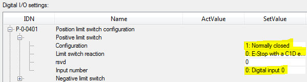
Expand Positive limit switch and set the following 3 parameters:
- Configuration
- Limit switch reaction
- Input number
Configuration and Input number are self-explanatory. For the Limit switch reaction, note that Beckhoff drives categorize events into 3 categories: Class 1 Diagnostic (fault), Class 2 Diagnostic (warning), and Class 3 Diagnostic (status), a.k.a. C1D, C2D, and C3D.
Simply, C1D is a “drive shut down” error, kicks the drive out of OP mode into ErrSafe-OP mode, and requires you to execute a drive reset command to clear the error (from the PLC, this is accomplished with an FB_SoEReset). This seems rather harsh for an overtravel limit fault, which really isn’t an internal drive, motor, or feedback error. I lean towards using a C2D warning, with an E-Stop. Ultimately it’s up to you to choose a reasonable configuration. Does a Hardware Limit Switch fault in your application indicate something internal has malfunctioned?
For selecting E-Stop vs. Axis halt, this refers to programmable error reactions. In the Drive Manager tab, go to the Channel A->Configuration->Error reaction / drive Halt node in the tree:
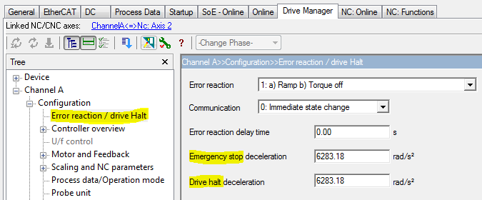
Here you can set your deceleration rates in the event of an E-Stop or Drive Halt error reaction.
Online Mode and Jogging
If you happen to have your I/O and drive (with motor) connected right now, you can actually activate the configuration and jog the motor back and forth with the built-in manual controls.
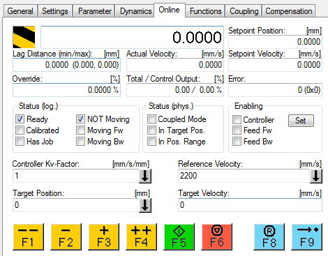
Assuming you’ve activated the configuration, in Solution Explorer, go to MOTION->NC Task 1 SAF->Axes and double-click on the axis node. Now go to the Online tab:
First you have to enable the axis. This means turning on the feedback loops within the drive, and turning on torque (i.e. current) to the motor. Note that when you do this, you will be causing motion, so make absolutely sure that no dangerous motion can result before you do this. To enable the axis, click the Set button inside the Enabling group box. That will display the Set Enabling dialog box:
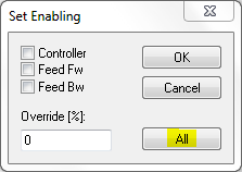
Click the All button. That’s a shortcut to enable the controller, the forward direction, the backward direction, and set the speed override to 100%. If successful, the drive will be enabled and the Online tab will look like this:
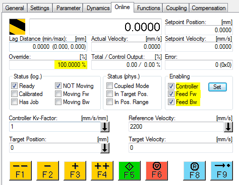
Now to test the axis, you can use the manual slow buttons (F2 and F3) at the bottom to “jog” the axis. When you do that, the motor should move, and the position number at the top of the screen should change to indicate the actual position.
If you have the limit switches installed, this is a good time to test them out. Jog towards a limit and make sure the axis responds appropriately when it reaches the sensor.
If your axis is hooked up to the actual load, now is the time to do some initial “tuning” of the axis. Most tuning is simply choosing appropriate maximum values for acceleration, deceleration, and jerk on the axis Parameter tab. It’s sometimes helpful to setup a repeating back-and-forth motion while you try changing the parameters.
Using the axis Functions tab, you can create a Reversing Sequence:
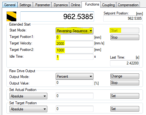
Remember that your axis hasn’t been “homed” (a.k.a. “referenced”) yet, so the positions are based on where the axis was when it started up. Make sure that you can safety move to the desired positions without hitting an end stop before you start the reversing sequence. Start with a shorter move and move it up from there.
You want to modify the acceleration, deceleration, and jerk parameters so that you get a fast response without unacceptable overshoot. Remember that at no time should you exceed the maximum velocity and torque capabilities of your mechanical system.
TwinCAT 3 comes with a really good oscilloscope-like tool called the TwinCAT 3 Scope. You create one by adding a TwinCAT 3 Measurement project under the solution in the Solution Explorer. I won’t go into the Scope now, but it’s a useful tool when trying to optimize a motion axis.
If you want to play around with the axis Online tab but you don’t have the physical I/O or drive connected, don’t worry. If your axis isn’t linked to the drive, or if you disable the drive, then TwinCAT 3 treats it as a simulated axis. You can do everything you would do with a normal drive and motor, and TwinCAT 3 will simulate an actual position that’s equal to the commanded position. This is really useful for simulating your system offline before you start it up in the field.
Manually Releasing a Brake
Some servo motors come with an optional motor brake. Some systems may have an external brake. In both cases the drive itself controls the brake output directly, energizing it to release the brake mechanism. The drive makes sure that torque is applied to the servo motor before releasing the brake, so the axis doesn’t fall or move unexpectedly.
In some cases you want to be able to manually release the brake for maintenance tasks. Before explaining this procedure, you must understand that this is situation-specific. If there’s any residual force on the axis, or if the axis carries a vertical load and will fall under gravity if you release the brake, then uncontrolled motion will occur when you release the brake. It is your responsibility to make the system safe before you release the brake. This might including blocking a vertical axis mechanically so it can’t fall, or releasing stored potential energy such as air before unlocking the brake.
The manual brake release function is in the Drive Manager tab of the physical drive node in the I/O list. In the tree, go to Channel A->Service Functions->Manual brake control. There you have the options for Automatic, Force lock and Force unlock.
Linking the Axis to the PLC
We’ve already seen how the NC task’s axis node links to the physical drive. Now we need to link the axis to the PLC. The first thing you have to do in your PLC is add a reference to the Tc2_MC2 library. In Solution Explorer, go to PLC->PLC1->PLC1 Project and right click on the References node. (That assumes your PLC project is called PLC1.) Click Add library… from the context menu to open the Add Library dialog. You can find the Tc2_MC2 library under Motion->PTP in the tree.
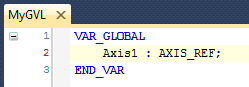
Next you need to define a variable of type AXIS_REF in your PLC project (typically in a global variable list):
Now build your PLC project (right click on the PLC1 Project node in Solution Explorer and choose Build from the context menu).
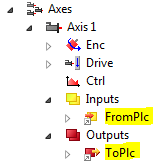
Now the Axis1 variable will be available for linking to the axis in the NC task. Double-click on the axis under the Axes node in the NC task and go to the Settings tab:
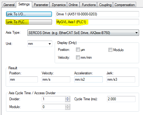
Click the Link To PLC… button to open the Select Axis PLC Reference dialog:
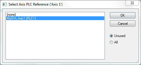
Select the line that says MyGVL.Axis1 and click OK. Now you’ve linked the axis to your PLC. This actually creates I/O linking between the PLC task and the axis in the NC task:
Make sure you activate this configuration before continuing.
Enabling the Axis
You use the MC_Power function block to enable an axis from the PLC:
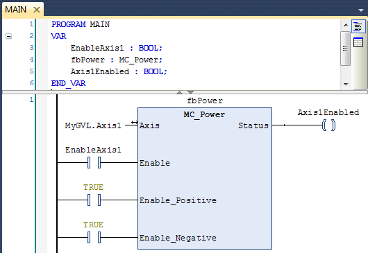
In this example, set EnableAxis1 to TRUE and if the function block is successful, the Axis1Enabled coil will be set to TRUE. If it won’t enable, the MC_Power function block has diagnostic outputs: Error and ErrorID. If you do get an error, you can find more information about the error codes by searching the internet for TwinCAT NC Error Codes.
Jogging the Axis
Use the MC_Jog function block to jog the axis from the PLC:
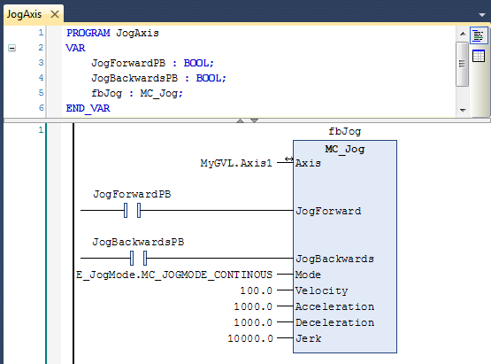
Make sure you choose sensible values for Velocity, Acceleration, Deceleration and Jerk.
You would normally connect JogForwardPB and JogBackwardsPB to physical button inputs or momentary buttons on your HMI. The axis will jog as long as you hold down on the button. Note that in almost all cases you should condition the JogForward and JogBackwards inputs so that they only work if you have the machine in manual mode.
Also note that this block can also perform incremental jog operations (where you move a specific amount with each button push). To implement incremental jog, change the Mode input to E_JogMode.MC_JOGMODE_INCHING and set the Position input to the amount you’d like to move with each button press. If you want to implement both modes and give the operator the ability to switch between modes, make sure you only use one MC_Jog block and just change the Mode input based on the operator’s selection.
Homing the Axis
Use the MC_Home function block to home (a.k.a. “reference”) the axis to a known position:
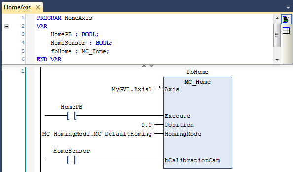
Similar to jogging, you should condition the Execute input with your manual mode signal, so the axis can only be homed if the machine is in manual mode.
When you execute the home function by pressing the HomePB momentary button, the axis will start moving towards the home sensor. When the sensor turns on, it will stop and move off the sensor slowly to record the exact encoder raw value when the input turns off. Once it turns off, the axis position will change to the position given in the Position input of the block.
In order to make this work, it’s best to implement the home sensor as a normally open switch positioned near the end of the travel. It needs to be built mechanically so that the sensor state is “on” if you’re on one side of it and “off” if you’re on the other side. The logic of MC_Home uses the initial sensor state to determine which direction to start moving to look for the sensor “edge”. You can change the direction and speeds of the homing sequence in the Parameter tab of the axis. I suggest setting the speed towards the sensor reasonably high, and the speed off the sensor to be slow, as this will allow it to find the sensor quickly, but still obtain good accuracy when finding the sensor edge.
Reading the Axis Status
If you want to know whether the axis has been homed, or if you want any kind of information about the axis status, use the MC_ReadStatus function block:
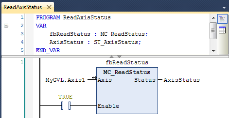
This block can be called constantly (once per scan) and the resulting variable AxisStatus contains a lot of interesting information about the state of the axis right now. Also, once you’ve called this function, it also updates the MyGVL.Axis1.Status variable with the same value, which you can use anywhere in your logic.
Moving the Axis to an Absolute Position
Now that the axis is referenced, you can command it to move to an absolute position with the MC_MoveAbsolute function block:
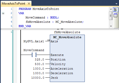
Make sure that MoveCommand is conditioned with the MyGVL.Axis1.Status.Homed status signal. You don’t want to try to move to an absolute position if you haven’t homed the axis yet.
When the block sees a rising edge on the Execute input, it will initiate a move to the given Position using the given motion parameters (Velocity, Acceleration, Deceleration, and Jerk). Note that turning off the Execute input does not stop the motion. You must use MC_Halt or MC_Stop to do that.
The reason is that when the rising edge happens on Execute, it pre-computes a desired motion profile for the axis and the NC task starts feeding this commanded position to the drive over the time period of the motion profile. The only way to change this motion profile is by executing a different function block. For instance, you can execute another MC_MoveAbsolute block to “change your mind” on the fly and send the axis to another final position. The NC task will compute a blended motion profile to move the axis to the new position. You could also execute an MC_Stop function block which will re-compute the motion profile to bring the axis to a stop.
What this means is that your PLC program must “remember” what you’ve commanded the axis to do so that you can take appropriate action by issuing new commands if the situation changes. For instance, if someone opens a guard door, you may be allowed a short amount of time where you have to decelerate to a stop under power before the safety system will drop out power to your drive. This is the responsibility of the PLC programmer to make sure this action happens. The only action the safety system can take is removing power, it can’t enforce a deceleration.
Conclusion
Obviously motion control is a big topic, and I’ve only introduced the subject and how it relates to TwinCAT 3 here. I hope this will be enough to get your axes moving and head you in the right direction. Please understand that motion control is complicated and requires a lot of experience. If you’re stuck on some technical detail, don’t be afraid to contact Beckhoff’s technical support. In my experience they’re very knowledgeable and helpful.
This chapter is part of the TwinCAT 3 Tutorial. Continue to the next chapter: Introduction to TwinSAFE.